Monetary velocity is an important, often ignored number that is an important determinant of GDP (gross domestic product) in an economy. It represents how often, on average, each dollar in the economy is spent for final goods and services. This site describes exactly what economic events determine it, and why an economy can be harmed when different wealth groups in an economy hold money with different velocities. Average monetary velocity times the amount of total money in an economy determines nominal GDP. M x V = nominal GDP
Get PDF copy of this essay here
- Section 1 what in the economy causes monetary velocity to be what it is
- Section 2 economic consequences implied by the above analysis
- Section 3 bad effect on economy when monetary velocity among groups is different
SECTION 1: what in the economy causes monetary velocity to be what it is
Monetary velocity only counts money spent for final goods/services, and does not count dollars that are exchanged for any other reason, such as buying bonds or stocks, or making or receiving a loan, or exchanging 5 one dollar bills for a 5 dollar bill.
No one seems to have any difficulty visualizing what total money held M in an economy means. However it seems most are mystified by what force in the economy causes monetary velocity to be what it is. This site is here to clear up the mystery. Here’s what one, completely perplexed economic commentator recently said about monetary velocity:
To paraphrase the Dread Pirate Roberts, anyone who claims that she fully understands what drives money velocity “is either lying or selling something.” Technology certainly plays a role that is only dimly understood. But without question two key inputs are inflation expectations and the level of interest rates.
The first two sentences in this statement are completely silly as I hope to show by the simple explanation to be given. The description below will bring complete clarity to its meaning. The explanation that follows will make obvious why the above quote in the last sentence about inflation and interest rates is quite correct—no magic or difficult mathematical economic analysis will be required to understand why. But an additional factor affecting velocity will also become evident: velocity will decrease with the perceived higher risk for investing (or saving) money.
To quickly give away the answer: Monetary velocity is crowd sourced, by the combined choices made by each individual person in an economy. It has to do with each person’s decision for how much cash money each person decides to hold compared to how fast they spend such money in their possession. Each agent in the economy has their own speed of spending money. People who hold little money, and spend it very fast–have high velocity. Those that have a lot of money that they spend slowly have low velocity. When all individual choices are properly combined, this is the only factor that collectively determines the monetary velocity of an economy. This is the only site I know of that describes exactly how to combine all these choices that determine the monetary velocity of an entire economy.
First determine velocity and amount of cash for each individual separately in the economy: Everyone makes a choice about how much money they want to hold for their cash expenses. Not too much, and not too little. If too little, it can increase anxiety about having enough to cover ordinary expenses as they occur. If too much, that extra money could be of more benefit if invested, which would then earn some interest. However some who don’t trust investments to be safe may even hold much more than they need for expenses. Monetary velocity can be thought of as how rapidly it takes to spend the amount of cash you on average typically like to hold. If only a short amount of time, that would represent high velocity. It’s determined for each person by knowing two numbers:
- How much average cash money each agent decides to generally hold for expenses.
- How rapidly that person spends that quantity of money for such expenses.
Velocity is completely determined for one agent once you know how many months it takes to spend that average amount of cash money they typically hold. If it takes one month (1/12 of a year) to spend that much their velocity is 12. If they spend the same amount in just half a month (1/24 of a year), they are spending each dollar twice as fast, so their velocity is 24. If it takes 6 months, then their monetary velocity is much lower at 12/6 = 2.
It is pretty obvious that the amount of total money (M) in the economy is determined by adding together the money amounts all agents hold together, either in hand or as cash in the bank. But it’s a little trickier how to combine all those velocities to get the velocity for the entire economy. The formula below shows how to combine each person’s velocity into a single velocity number that describes the velocity of the complete economy.
That’s ALL there is to determine monetary velocity in an economy. It’s determined completely once you know everyone’s individual velocity, and also the amount of money they typically hold! This formula is derived a little further down the page.
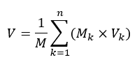
V = monetary velocity of M1 for entire economy
M = total M1 money in economy
Mk = individual M1 cash held for expenses by person k
Vk= individual velocity for cash held by person k
n = number of people in economy
What about banks? It’s worth noting that a few of these “people” are banks. They do hold reserves, but these are not counted as “money in circulation” so cash they hold does not affect velocity calculations.
What economic factors determine velocity? Now the question of “what in the economy determines monetary velocity” has been transformed to a simple question: “what factors affect people’s decisions about how much cash money they decide to hold to cover expenses?”
Or you could ask “what makes you decide how much money you should hold?” The question about velocity is no more (or less) complicated than answering that question.
What could make you want to hold more cash? The LOW velocity choice.
- Interest rates on saving cash as investment is too tiny to bother, so hold more safe cash instead
- You fear investments or loaning are risky, so hold more safe cash instead
- Interest rates may rise soon, hold cash money ready to invest later when interest rates rise.
- Inflation is low–no worries about money rapidly losing value.
What makes you want to hold less cash? The HIGH velocity choice.
- Interest rate on savings is very high. Hold less cash and invest (or loan) more to earn interest.
- No fear about safety of the investment or loan. Choose safe investment instead of holding money
- High inflation is happening. Spend quickly before its value disappears.
- Income low, very little cash for desired expenses. Living paycheck to paycheck.
SECTION 2: Economic consequences implied by the above analysis
- Monetary velocity is likely to be low if people are holding a lot of non transactional cash.
- Monetary velocity is correlated with interest rates; high interest discourages holding cash money.
- Monetary velocity is correlated with perceived safety of investment.
- Monetary velocity is correlated with high active inflation.
Prediction 1: Very low interest rates cause low velocity and thus reduce GDP. Here is empirical evidence for the assertion that interest rates strongly influence velocity: Thanks to Mr. Luci Benati, University of Bern for gathering this data into two informative pages. Graphs for ten different countries’ economies show both velocity and interest rates. Interest rates are shown in black. Velocity in red. Look at Figure 2a and Figure 2b just after page 10. Luci Benati-Money Velocity Link Note that velocity follows slightly behind interest rates.
Prediction 2: Japan was the first country to reduce interest rates to unprecedented low levels in failed attempt to boost GDP from 2000 to 2017. With low interest reward on money the opportunity cost for holding cash was very low, therefore people held more money, velocity went down, therefore GDP barely moved contrary to the expected increase. The US and Europe experienced the same after 2010.
Prediction 3: Lowering interest rates too much to attempt to increase GDP is a very bad idea. Velocity, and therefore GDP both go to zip. The lowest advisable interest rate is also called the low interest rate bound for effective monetary policy.
The Math: Here is how this formula is derived. Each person’s contribution to GDP is equal to their individual monetary velocity times how much cash they hold: As expressed in this equation, GDP of an entire economy equals the sum of each person’s spending for goods and services. 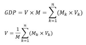
Math detail: Symbols in equation are defined in velocity equation above. Velocity can also be defined slightly differently. Instead of Vk being defined by the amount of time required for spending average held cash, Vk can be defined by the amount of time required to earn average held cash. For any individual, those two numbers won’t usually be exactly the same–except those living paycheck to paycheck. But in a closed economy the TOTAL economic velocity will be the same either way it’s calculated.
SECTION 3: bad effect on economy when monetary velocity among groups is different. A new way to explain the 1930’s depression.
Monetary velocity is normally a very boring statistic in an economy with homogenous agents–that is, in an economy where everyone spends and earns money about the same way. Since macroeconomic analysis commonly assumes one “average” agent, it isn’t surprising that velocity has been barely mentioned or noticed or thought to be significant by economists because a commonly used “single agent” model assumes that everyone holds cash with the same velocity.
It’s quite different and much more interesting in the actual US economy which is much more heterogenous with respect to total wealth. In 2020 a few high wealth individuals held a lot of cash that they were not spending, at low velocity. You can see such data for 2022 in the chart below “WEALH CATEGORY”: The top 1% held 31% of total cash, likely at low velocity, which could be called a “liquidity trap” by Keynes. At the same time a much larger, lower wealth group held money which is spent with higher velocity. When a few hold lots of money which is not being spent, money quantity is effectively reduced for the many others in the economy, reducing money supply and GDP for the much larger group who buy most of the goods/services, which therefore reduces GDP.
An economy with heterogenous agents with some wealthy individuals holding high cash has the same effect on the economy as the FED when it deliberately slows an economy by shrinking the money supply. The FED actually removes cash from the economy. Wealthy individuals holding a lot of money as wealth and not spending are essentially taking it out of circulation. Either method depresses GDP in a similar way by reducing circulating cash in the economy. One difference between those two methods is the effect on interest rates. When the FED takes money out completely, that typically is intended to raise interest rates. The money they remove also reduces money available to be borrowed. When money is held out by people just holding it for wealth storage, it is at least potentially still able to be borrowed, so that should not raise interest rates.
This is an unusual way to describe how wealth inequality can suppress an economy. I am suggesting that this is what caused the 1930’s depression. The far more usual explanation that economists use to try to explain how high income/wealth inequality could reduce GDP is to assume that those with higher wealth have lower MPC (marginal propensity to consume) which would cause reduced demand on the entire economy by only that small number who consume less percentage of their income than those of lower wealth. My description is unconventional in that it says that individuals holding high amounts of cash can slow the economy exactly how the FED does it: by taking money out of circulation. The FED does it literally by removing cash. High wealth individuals could hold high amounts of cash out of circulation that they are just holding as wealth. I believe this could have a much stronger effect than the common explanation of lower MPC by a relatively small number of wealthy consumers who consume at low monetary velocity. The economist Keynes also specifically mentioned this possibility for slowing an economy, which he called a “liquidity trap.”
Velocity, and therefore GDP, could shrink when interest rates are near zero, as more wealthy agents may decide to hold more cash because low interest causes low opportunity cost to hold cash, especially if lending is also riskier during a financial crisis. This shows how when interest rates are too low they can slow an economy rather than encourage it. Economists usually expect lower interest to increase GDP–but if it goes too low it could cause money to be held in a Keynes’ “liquidity trap.”
To examine this view quantitatively: In the US according to the FED Distributional Financial Accounts, the top 1% wealth group holds 31% of all cash held by consumers ($1.2T). Since that 1% of population likely doesn’t spend 31% of the GDP, much of this cash is likely not used for transactions, but just as one way to hold static precautionary wealth. This would likely reduce transactional cash to reduce velocity and GDP in an economy.
Unfortunately the FED does not measure velocity or spending GDP separately for different wealth categories so vital data is missing to evaluate whether this hypothesis is true. The FED does measure money holdings for different wealth groups: specifically the top 1%, 90-99%, 50-90%, 0-50%–but to my knowledge they do not measure velocity, or equivalently the amount these groups spend for goods/services. Data in table below is from FRED, Distributional Financial Accounts, Q1 of 2022.
| WEALTH CATEGORY | % of total cash: Checkable deposits and currency in 2022 | % spending of GDP | Monetary velocity |
| Top 1% | 31% | ? | ? |
| 90-99% | 35% | ? | ? |
| 50-90% | 27% | ? | ? |
| 1-50% | 6.4% | ? | ? |
Hypothesis: Based on this idea here is a new explanation for how this could explain why the 1929 stock market crash could have also crashed spending, exacerbating the depression in 1930’s. Most economists have claimed that the stock market crash could not have caused the 1930’s depression. Their argument is that only a small percentage of people owned stock in 1929 who directly lost wealth–and that small number was not large enough to have enough effect on consumption that could have caused such depression.
Why I believe there is a possible better explanation: Total M2 cash in 1929 was $45 billion. Before the crash the stock market capitalization value had far greater market value at $87 billion, and because the stock market was rapidly rising this meant money had a high opportunity cost to hold, encouraging the wealthy to not hold much cash tending to keep their cash volume low, and velocity high. After the crash, stocks dropped by $19 billion and cash was suddenly likely seen by those few with high stock wealth more desirable to hold–and stocks much less–likely pulling in a significant amount of the $45 billion cash to be held by the 4% that had previously held $87 billion worth of stock–who now found cash much more desirable to hold. Because of the great wealth disparity at the time, the above explanation could explain how this could have sucked significant formerly transactional cash out of the economy from low wealth people as low velocity precautionary cash become increasingly held by those of high wealth–which could have created a “liquidity trap.”
Note that when money is often said to “go into” the stock market it does not really go “into” stocks. Such money is almost always just a transfer of money from one stock buyer to seller–after which the seller could be eager to quickly get rid of newly acquired cash by purchasing another stock with more prospects. That is how money stays at high velocity.
After the crash a lot of stock market value must have gone into low velocity cash. How much is anybody’s guess. The stock market value dropped in a very short time by $19B. Many would have liked to convert all their stock value to cash, but of course in many cases that was not possible as stocks became rapidly less valuable. Perhaps it is not an unreasonable wild guess that perhaps $10 billion more cash might have been attracted to suddenly be held in lieu of stock wealth that declined which could have reduced GDP by 20%.
.